1  part-to-whole

Explore the relationship between a whole and its components, showcasing proportions and percentages. Ideal for visualizing contributions of individual elements to the overall entity.

library(tidyverse)

Warning: package 'dplyr' was built under R version 4.2.3

Warning: package 'stringr' was built under R version 4.2.3

── Attaching core tidyverse packages ──────────────────────── tidyverse 2.0.0 ──
✔ dplyr     1.1.4     ✔ readr     2.1.4
✔ forcats   1.0.0     ✔ stringr   1.5.1
✔ ggplot2   3.4.4     ✔ tibble    3.2.1
✔ lubridate 1.9.3     ✔ tidyr     1.3.0
✔ purrr     1.0.2     
── Conflicts ────────────────────────────────────────── tidyverse_conflicts() ──
✖ dplyr::filter() masks stats::filter()
✖ dplyr::lag()    masks stats::lag()
ℹ Use the conflicted package (<http://conflicted.r-lib.org/>) to force all conflicts to become errors

library(dplyr)
library(ggplot2)
library(ggrepel)

data <- read.csv("dataset/insurance.csv")

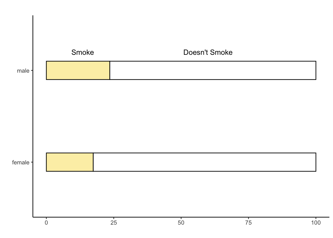
type.cols <- c("no" = "white",
               "yes" = "#fcefb4")
data %>%
    group_by(sex, smoker) %>%
    summarise(count = n()) %>%
    mutate(percentage = count / sum(count) * 100) %>%
    ggplot(aes(x = percentage, y = sex, fill = smoker)) +
    geom_bar(stat = "identity", position = "stack", color = "black", width=0.2) +
  annotate(geom = "text", x = 13.5, y = 2.2, label = "Smoke")+
  annotate(geom = "text", x = 60, y = 2.2, label = "Doesn't Smoke")+
    scale_fill_manual(values = type.cols) +  # Manually set fill colors
    ylab("") +
  labs(title = "")+
    xlab("") +
    guides(fill = guide_legend(title = "Type", override.aes = aes(label = ""))) +
    theme_classic() +
  theme(legend.position = "none")

`summarise()` has grouped output by 'sex'. You can override using the `.groups`
argument.