library(tidyverse)10 hybrid
Combination of chart type
10.1 Setup
10.2 Creating dataset
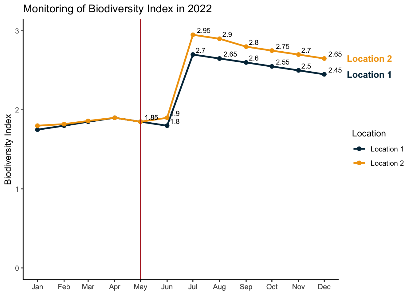
# Create example data for location 1
location1 <- data.frame(date = seq(as.Date("2022-01-01"), by = "month", length.out = 12),
                        index = c(1.75, 1.80, 1.85, 1.90, 1.85, 1.80, 2.70, 2.65, 2.60, 2.55, 2.50, 2.45))

# Create example data for location 2
location2 <- data.frame(date = seq(as.Date("2022-01-01"), by = "month", length.out = 12),
                        index = c(1.80, 1.82, 1.86, 1.90, 1.85, 1.90, 2.95, 2.90, 2.80, 2.75, 2.70, 2.65))

# Combine data for both locations into a single dataframe
biodiversity_data <- data.frame(location = c(rep("Location 1", 12), rep("Location 2", 12)),
                                date = c(location1$date, location2$date),
                                index = c(location1$index, location2$index))
10.3 Data visualization
loc.cols <- c("Location 1" = "#023047", "Location 2" = "#f1a208")
ggplot(data = biodiversity_data, aes(x = date, y = index, color = location)) +
  geom_line(linewidth = 1) +
  geom_point(size = 2) +
  labs(x = NULL, y = "Biodiversity Index", color = "Location") +
  ggtitle("Monitoring of Biodiversity Index in 2022") +
  geom_text(data = biodiversity_data[biodiversity_data$date >= "2022-05-01" &
                                       biodiversity_data$location == "Location 1",],
            aes(label = index), hjust = -0.3, vjust = -0.4, size = 3, color = "black") +
  geom_text(data = biodiversity_data[biodiversity_data$date >= "2022-05-01" &
                                       biodiversity_data$location == "Location 2",],
            aes(label = index), hjust = -0.3, vjust = -0.4, size = 3, color = "black")+
  scale_color_manual(values = loc.cols)+
  theme_classic()+
  annotate(geom="text", y=2.65, x=c(as_date("2022-12-01")), label="Location 2",
             color="#f1a208", hjust = -0.5, fontface = "bold")+
    annotate(geom="text", y=2.45, x=c(as_date("2022-12-01")), label="Location 1",
             color="#023047", hjust = -0.5, fontface = "bold")+
  theme(legend.position = "right")+
  scale_x_date(date_labels = "%b", breaks = biodiversity_data$date)+
    coord_cartesian(ylim=c(0,3),clip="off")+
    geom_vline(xintercept = c(as_date("2022-5-01")), color = "firebrick")